Finding gendered words
Overview
In this vignette, we will look for gender-associated words We will do this by looking for words that follow the pronoun “she” more often than “he”, or vice-versa. The vignette is based on Julia Silge’s blog post, “Gender roles with text mining and n-grams”.
We will use the corpus package, but not rely on any other external dependencies. The set-up is as follows.
library("corpus")

# colors from RColorBrewer::brewer.pal(6, "Set1")
palette(c("#E41A1C", "#377EB8", "#4DAF4A", "#984EA3", "#FF7F00", "#FFFF33"))

# ensure consistent runs
set.seed(0)
Gender bigrams in Austen’s novels
We will be studying gender in the context of Jane Austen’s completed novels, downloaded from Project Gutenberg.
# Gutenberg IDs gotten from gutenbergr::gutenberg_works(author == "Austen, Jane")
(austen <- gutenberg_corpus(c(161, 1342, 141, 158, 121, 105)))
Determining mirror for Project Gutenberg from https://www.gutenberg.org/MIRRORS.ALLUsing mirror http://aleph.gutenberg.org/Converting text from declared encoding "ISO-8859-1" to UTF-8 title author language text
1 Sense and Sensibility Jane Austen English SENSE AND SENSIBILITY\n\nby Jane Austen\n\n(1811)…
2 Pride and Prejudice Jane Austen English PRIDE AND PREJUDICE\n\nBy Jane Austen\n\n\n\nChap…
3 Mansfield Park Jane Austen English MANSFIELD PARK\n\n(1814)\n\n\nBy Jane Austen\n\n…
4 Emma Jane Austen English EMMA\n\nBy Jane Austen\n\n\n\n\nVOLUME I\n\n\n\nC…
5 Northanger Abbey Jane Austen English NORTHANGER ABBEY\n\n\nby\n\nJane Austen (1803)\n…
6 Persuasion Jane Austen English Persuasion\n\n\nby\n\nJane Austen\n\n(1818)\n\n\n…For tokens, we will be using the lower-cased non-punctuation words
text_filter(austen)$drop_punct <- TRUESpecifically, we will look at the bigrams from these novels where the first type is a pronoun.
pronouns <- c("he", "she")
bigram_counts <- term_stats(austen, ngrams = 2, types = TRUE,
                            subset = type1 %in% pronouns)
print(bigram_counts)
term type1 type2 count support
1 she had she had 1472 6
2 she was she was 1377 6
3 he had he had 1023 6
4 he was he was 889 6
5 she could she could 817 6
6 he is he is 399 6
7 she would she would 383 6
8 she is she is 330 6
9 he could he could 307 6
10 he would he would 264 6
11 she did she did 227 6
12 he has he has 222 6
13 he did he did 195 6
14 she felt she felt 189 6
15 she must she must 184 6
16 she might she might 173 6
17 he should he should 158 6
18 she has she has 149 6
19 he must he must 143 6
20 he might he might 137 6
⋮ (1573 rows total)Above, we can see the most common bigrams with gendered pronouns as their first types.
Next, we rearrange the data into tabular form, with one row for each term and one column for each pronoun:
terms <-  with(bigram_counts,
               tapply(count, list(type2, type1), identity, default = 0))
head(terms)
he she
_did_ 4 1
_had 1 0
_had_ 2 4
_is_ 0 1
_may_ 1 0
_meant_ 0 1It looks like some terms get emphasized in the text by underscores. We can investigate some of these:
# inspect a random sample of the occurrences
text_sample(austen, c("_did_", "_had", "_meant_"))
text before instance after
1 3 …rprise to herself. And the\nnext day _did_ bring a surprise to her. Henry had sa…
2 2 …ome,” cried Elizabeth; “perhaps she\n _meant_ well, but, under such a misfortune as…
3 2 …ad been brought on by himself. If he _had another_\nmotive, I am sure it would …
4 2 … would never come back again. People _did_ say\nyou meant to quit the place enti…
5 3 … he\nis Henry, for a time.”\n\nJulia _did_ suffer, however, though Mrs. Grant di…
6 2 …red her--indeed I rather believe he\n _did_ --I heard something about it--but I ha…
7 2 …humour encouraged, yet, whenever she _did_ speak, she must be vulgar.\nNor was h…
8 3 …he others prepared to begin.\n\nThey _did_ begin; and being too much engaged in …
9 4 …in her own mind, determined that he _did_ know what he was talking\nabout, and …
10 2 …the\nfirst, you may remember.”\n\n“I _did_ hear, too, that there was a time, whe…
11 2 …ced with her twice. To be\nsure that _did_ seem as if he admired her--indeed I r…
12 3 …found, from Edmund’s manner, that he _did_ mean to\ngo with her. He too was taki…
13 2 …y evident whenever they met, that he _did_ admire her and\nto _her_ it was equal…
14 3 …e\nheard of beyond themselves. Julia _did_ seem inclined to admit that\nMaria’s …Let’s clean the terms by removing underscores, and recompute the counts:
terms <-  with(bigram_counts,
               tapply(count, list(gsub("_", "", type2), type1),
                      sum, default = 0))
head(terms)
he she
a 5 6
able 0 1
abominates 1 0
absented 0 1
absolutely 3 1
abstained 0 1Here, we changed the aggregation function from identity() to sum() to sum the counts over all types that are equal after removing underscores.
Gender-specific usage rates
We want to find terms that are associated with particular gendered pronouns. As an example, take term “loves”:
term <- "loves"
i <- match(term, rownames(terms))
tab <- cbind(terms[i,], colSums(terms[-i,]))
colnames(tab) <- c(term, paste0("\u00ac", term))
print(tab)
loves ¬loves
he 5 7287
she 7 10130When the first type in a bigram is “he”, it is followed by “loves” in 5 instances and another type in 6988 instances. Here are the relative rates of “loves”, conditional on the first type in the bigram:
(rates <- tab[,"loves"] / rowSums(tab)) he she
0.0006856829 0.0006905396 The ratio of these rates is very close to one:
rates[["she"]] / rates[["he"]][1] 1.007083The log (base-2) ratio of the rates is close to zero:
log2(rates[["she"]]) - log2(rates[["he"]])[1] 0.01018254This log ratio is a good measure of the strength of association. When the value is close to zero, there is no meaningful association. For large absolute log ratios, we would say that there is a meaningful difference in usage between the genders.
We compute the log ratios for all types. To avoid dividing by zero, and to smooth the estimates when the counts are small, we add 0.5 to the count when estimating the rate. (Many people smooth by adding 1, but I prefer 0.5 since that value has stronger theoretical justification.)
Some terms only appear once in the corpus. The rate estimates for these terms will be unreliable, so we discard them.
tot <- colSums(terms)
common_terms <- terms[rowSums(terms) > 1,]
he  <- (common_terms[,"he"] + 0.5) / (tot[["he"]] + 1)
she <- ((common_terms[,"she"] + 0.5) / (tot[["she"]] + 1))
log2_ratio <- log2(she) - log2(he)
Here are a histogram and normal probability plot of the estimates for the remaining terms.
par(mfrow = c(1, 2))
hist(log2_ratio, breaks = "Scott", col = 2, border = "white")
qqnorm(log2_ratio, col = 2)
qqline(log2_ratio, col = 1, lty = 2)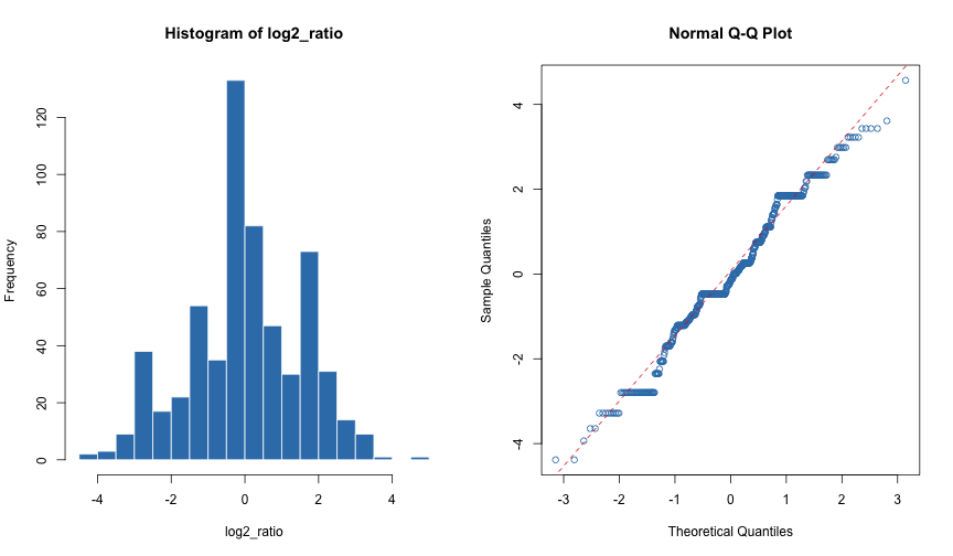
Rate Ratio Estimates
This doesn’t quite look like a normal, but the distribution is symmetric, and the tails are about as heavy as those of a normal. So, the z-score will be a reasonable measure of how typical or unusual each log rate is.
z <- (log2_ratio - mean(log2_ratio)) / sd(log2_ratio)Here are the words more than two standard deviations away from the mean log ratio:
sort(log2_ratio[abs(z) > 2]) gravely smiling no indeed turning addressing believes bowed
-4.382079 -4.382079 -3.934620 -3.645114 -3.645114 -3.282544 -3.282544 -3.282544
intends next perhaps quite sought won't beheld lay
-3.282544 -3.282544 -3.282544 -3.282544 -3.282544 -3.282544 3.225251 3.225251
looks refused yet checked dreaded eagerly seized hurried
3.225251 3.225251 3.225251 3.431702 3.431702 3.431702 3.431702 3.612274
remembered
4.569205 The terms “remembered”, “hurried”, and “seized” have more “she” usages; the terms “gravely”, “believes”, and “bowed” have more “he” usages.
Uncertainty quantification
It’s hard to know which of these differences are meaningful without quantifying the error associated with the estimates. Some words are common, and we have reliable estimates of the log ratios. Other words are rare, and the estimates are based on a small number of occurrences. In the rare case, the estimates of the log ratios will be unreliable.
We need standard errors of our estimates. We can get these by starting with the proportion estimates he and she, and then applying the delta method.
The he and she rates are proportions. We get their standard errors by using the usual formula for the standard error of a proportion, based on the Binomial variance formula:
he_se <- sqrt(he * (1 - he) / tot[["he"]])
she_se <- sqrt(she * (1 - she) / tot[["she"]])
To find the standard errors for the logarithms of these quantities, we use the delta method. We multiply the standard error by the absolute value of the derivative of the logarithm function evaluated at the estimate:
log2_he_se <- abs(1 / (log(2) * he)) * he_se
log2_she_se <- abs(1 / (log(2) * she)) * she_se
These formulas follow from using a Taylor expansion of log2 around the estimate, using that the derivative of log2(x) is 1 / (log(2) * x).
Finally, for the standard error of log2_ratio, we assume that the log2_he and log2_she estimates are approximately independent, so that the variance of their difference is the sum of their variances. This gives a formula for the standard error of the log ratio:
log2_ratio_se <- sqrt(log2_he_se^2 + log2_she_se^2)Here are all of the estimated log ratios, along, with error bars for those that are statistically significantly different from zero.
# put the estimates in increasing order
r <- rank(log2_ratio, ties.method = "first")

# find the statistically significant cases
signif <- (abs(log2_ratio) / log2_ratio_se > 2)
i <- signif

# set up the plot
xlim <- xlim <- range(r)
ylim <- range(log2_ratio,
              (log2_ratio - log2_ratio_se)[i],
              (log2_ratio + log2_ratio_se)[i])
plot(xlim, ylim, type = "n", xlab = "Rank",
     ylab = expression(paste(Log[2], " (She / He) Usage Rate")))

# horizontal line at zero
abline(h = 0, col = "gray", lty = 2)

# standard error around interesting points
segments(r[i], (log2_ratio - log2_ratio_se)[i],
         r[i], (log2_ratio + log2_ratio_se)[i])
segments((r - 0.4)[i], (log2_ratio - log2_ratio_se)[i],
         (r + 0.4)[i], (log2_ratio - log2_ratio_se)[i])
segments((r - 0.4)[i], (log2_ratio + log2_ratio_se)[i],
         (r + 0.4)[i], (log2_ratio + log2_ratio_se)[i])

# points at the estimates
points(r, log2_ratio, col = 2, cex = 0.5)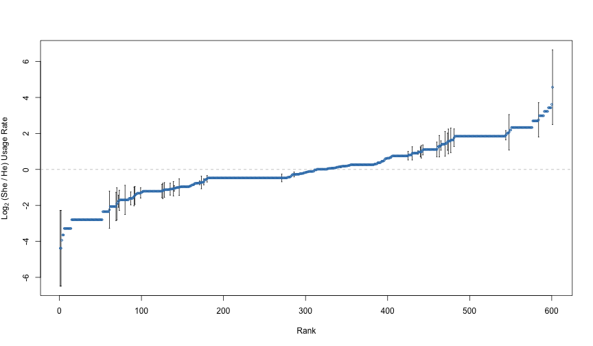
Rate Ratio Estimates, with Error Bars
Notice that many of the more extreme estimates are not statistically significant. One word with a large estimate not deemed statistically significant is the word “expressed”. Here are the counts for that word, along with the log ratio estimate and standard error:
print(terms["expressed",]) he she
9 5 print(log2_ratio[["expressed"]])[1] -1.263685print(log2_ratio_se[["expressed"]])[1] 0.7727217This is a word with a large imbalance, but only in a relatively small number of samples. Due to the lack of data for the word “expressed”, we deem this imbalance to not be statistically significant. Compare this to the word “felt”:
print(terms["felt",]) he she
36 189 print(log2_ratio[["felt"]])[1] 1.901041print(log2_ratio_se[["felt"]])[1] 0.2598566This has an effect size estimate on the same order as “stopped”, but the estimate is much more reliable given the larger number of appearances of the word “felt”. We judge “felt” both to have a practically significant difference and a statistically significant difference.
The word “was” exhibits one other extreme:
print(terms["was",]) he she
891 1378 print(log2_ratio[["was"]])[1] 0.1536038print(log2_ratio_se[["was"]])[1] 0.0579161This word has only a minor difference between “he” and “she”, but it shows up often enough for us to get a reliable estimate of the difference. The word “was” has a statistically significant difference between the genders, but probably not a practically significant difference.
In the context of our application, a word is practically significance if the absolute value of its estimate is large. This difference is statistically significant if the estimate is large relative to its standard error. If we only care about Austen’s writing in these six novels, we may not care about statistical significance. If, however, we want to make a statement about Austen’s writing style in general, then we want to generalize beyond our data set, and we should only do so for words we can get reliable estimates for.
Results
Here are the estimates for the words with statistically significant gender imbalances, defined s having an estimated log ratio more than two standard errors away from zero.
# order by log ratio, then name
o <- order(log2_ratio, names(log2_ratio))
est <- log2_ratio[o]
se <- log2_ratio_se[o]

# only keep statistically significant cases
signif <- (abs(est) / se > 2)
est <- est[signif]
se <- se[signif]

# find practically significant cases
pract <- abs(est) > 1

# get the terms
term <- names(est)
i <- seq_along(term)

# set up the plot
par(mar = c(5, 6, 2, 2) + 0.1)
xlim <- range(est - se, est + se)
ylim <- range(i)
plot(xlim, ylim, type = "n",
     xlab = "Relative appearance after 'she' compared to 'he'",
     ylab = "", axes = FALSE)

# x-axis
ticks <- seq(-3, 6)
labels = paste0(2 ^ ticks, "x")
labels[ticks == 0] <- "Same"
axis(1, at = ticks, labels = labels)
abline(v = ticks, col = "gray", lwd = 0.5)

# y-axis, with term labels
axis(2, at = i, labels = term, las = 1)
abline(h = i, lty = 3, col = "gray")

# frame the plot
box()

# standard errors
col <- ifelse(est > 0, 3, 4)
segments(est - se, i, est + se, i, lwd = 1.5, col = col)
segments(est - se, i - 0.2, est - se, i + 0.2, lwd = 1.5, col = col)
segments(est + se, i - 0.2, est + se, i + 0.2, lwd = 1.5, col = col)

# estimates
points(est, i, pch = 16, cex = 0.75, col = col)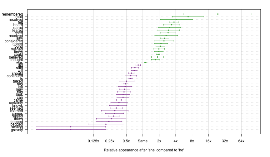
Statistically Significant Gender Imbalances
Not all of these are practically significant. Words like “should”, “will”, and “was” show up because they are common, and it is possible to get precise estimates of their gender imbalances. Still, we can see many examples of words that have both statistically and practically meaningful gender imbalances, especially “she”-slanted words like “remembered”, “read”, “resolved”, and “felt”.
In Silge’s original analysis, she used an ad-hoc filter of statistical significance, considering only words that appeared more than 10 times in the corpus. Her filter does a reasonable job of removing spurious results. Indeed, her list of the most gender-associated words mostly agrees with those reported here. There are, however, some notable differences. Silge’s list of “he” words does not include “begged”, but it does include “stopt”, “shook”, “expressed”, and “wants”. Similarly, Silge’s list of top “she” words includes some words that are excluded here: “longed”, “instantly”, “expected”, “ran” and “caught”.
I suspect that many of the words here have gender imbalances simply because the protagonists are female. The novels give us insights into the protagonists’ emotional states, but not into those of the supporting characters. It would be nice if we could get more balanced comparison by adjusting for the genders of the protagonists. Until we do that, it’s hard to know if there’s anything meaningful in these differences.