Introduction to corpus
Overview
This vignette demonstrates the functionality provided by the corpus R package. The running example throughout is an analysis of the text of L. Frank Baum’s novel, The Wonderful Wizard of Oz.
Setup
We load the corpus package, set the color palette, and set the random number generator seed. We will not use any external packages in this vignette.
library("corpus")

# colors from RColorBrewer::brewer.pal(6, "Set1")
palette(c("#E41A1C", "#377EB8", "#4DAF4A", "#984EA3", "#FF7F00", "#FFFF33"))

# ensure consistent runs
set.seed(0)
Data preparation
The The Wonderful Wizard of Oz is available as Project Gutenberg EBook #55. We first download the text and strip off the Project Gutenberg header and footer.
url <- "http://www.gutenberg.org/cache/epub/55/pg55.txt"
raw <- readLines(url, encoding = "UTF-8")

# the text starts after the Project Gutenberg header...
start <- grep("^\\*\\*\\* START OF THIS PROJECT GUTENBERG EBOOK", raw) + 1

# ...end ends at the Project Gutenberg footer.
stop <- grep("^End of Project Gutenberg", raw) - 1

lines <- raw[start:stop]
The novel starts with front matter: a title page, table of contents, introduction, and half title page. Then, a series of chapters follow. We group the lines by section.
# the front matter ends at the half title page
half_title <- grep("^THE WONDERFUL WIZARD OF OZ", lines)

# chapters start with "1.", "2.", etc...
chapter <- grep("^[[:space:]]*[[:digit:]]+\\.", lines)

# ... and appear after the half title page
chapter <- chapter[chapter > half_title]

# get the section texts (including the front matter)
start <- c(1, chapter + 1) # + 1 to skip title
end <- c(chapter - 1, length(lines))
text <- mapply(function(s, e) paste(lines[s:e], collapse = "\n"), start, end)

# trim leading and trailing white space
text <- trimws(text)

# discard the front matter
text <- text[-1]

# get the section titles, removing the prefix ("1.", "2.", etc.)
title <- sub("^[[:space:]]*[[:digit:]]+[.][[:space:]]*", "", lines[chapter])
title <- trimws(title)
Corpus object
Now that we have obtained our raw data, we put everything together into a corpus data frame object, constructed via the corpus_frame() function:
data <- corpus_frame(title, text)

# set the row names; not necessary but makes results easier to read
rownames(data) <- sprintf("ch%02d", seq_along(chapter))
The corpus_frame() function behaves similarly to the data.frame function, but expects one of the columns to be named "text". Note that we do not need to specify stringsAsFactors = FALSE when creating a corpus data frame object. As an alternative to using the corpus_frame() function, we can construct a data frame using some other method (e.g., read.csv or read_ndjson) and use the as_corpus_frame() function.
A corpus data frame object is just a data frame with a column named “text” of type "corpus_text". When using the corpus library, it is not strictly necessary to use corpus data frame objects as inputs; most functions will accept with character vectors, ordinary data frames, quanteda corpus objects, and tm Corpus objects.. Using a native corpus object gives better printing behavior and allows setting a text_filter attribute to override the default text preprocessing.
print(data) # better output than printing a data frame, cuts off after 20 rows title text
ch01 The Cyclone Dorothy lived in the midst of the great Kansas prairies…
ch02 The Council with the Munchkins She was awakened by a shock, so sudden and severe that …
ch03 How Dorothy Saved the Scarecrow When Dorothy was left alone she began to feel hungry. …
ch04 The Road Through the Forest After a few hours the road began to be rough, and the w…
ch05 The Rescue of the Tin Woodman When Dorothy awoke the sun was shining through the tree…
ch06 The Cowardly Lion All this time Dorothy and her companions had been walki…
ch07 The Journey to the Great Oz They were obliged to camp out that night under a large …
ch08 The Deadly Poppy Field Our little party of travelers awakened the next morning…
ch09 The Queen of the Field Mice "We cannot be far from the road of yellow brick, now," …
ch10 The Guardian of the Gate It was some time before the Cowardly Lion awakened, for…
ch11 The Wonderful City of Oz Even with eyes protected by the green spectacles, Dorot…
ch12 The Search for the Wicked Witch The soldier with the green whiskers led them through th…
ch13 The Rescue The Cowardly Lion was much pleased to hear that the Wic…
ch14 The Winged Monkeys You will remember there was no road--not even a pathway…
ch15 The Discovery of Oz, the Terrible The four travelers walked up to the great gate of Emera…
ch16 The Magic Art of the Great Humbug Next morning the Scarecrow said to his friends:\n\n"Con…
ch17 How the Balloon Was Launched For three days Dorothy heard nothing from Oz. These we…
ch18 Away to the South Dorothy wept bitterly at the passing of her hope to get…
ch19 Attacked by the Fighting Trees The next morning Dorothy kissed the pretty green girl g…
ch20 The Dainty China Country While the Woodman was making a ladder from wood which h…
⋮ (24 rows total)print(data, 5) # cuts off after 5 rows title text
ch01 The Cyclone Dorothy lived in the midst of the great Kansas prairies, …
ch02 The Council with the Munchkins She was awakened by a shock, so sudden and severe that if…
ch03 How Dorothy Saved the Scarecrow When Dorothy was left alone she began to feel hungry. So…
ch04 The Road Through the Forest After a few hours the road began to be rough, and the wal…
ch05 The Rescue of the Tin Woodman When Dorothy awoke the sun was shining through the trees …
⋮ (24 rows total)print(data, -1) # prints all rows title text
ch01 The Cyclone Dorothy lived in the midst of the great Kansa…
ch02 The Council with the Munchkins She was awakened by a shock, so sudden and se…
ch03 How Dorothy Saved the Scarecrow When Dorothy was left alone she began to feel…
ch04 The Road Through the Forest After a few hours the road began to be rough,…
ch05 The Rescue of the Tin Woodman When Dorothy awoke the sun was shining throug…
ch06 The Cowardly Lion All this time Dorothy and her companions had …
ch07 The Journey to the Great Oz They were obliged to camp out that night unde…
ch08 The Deadly Poppy Field Our little party of travelers awakened the ne…
ch09 The Queen of the Field Mice "We cannot be far from the road of yellow bri…
ch10 The Guardian of the Gate It was some time before the Cowardly Lion awa…
ch11 The Wonderful City of Oz Even with eyes protected by the green spectac…
ch12 The Search for the Wicked Witch The soldier with the green whiskers led them …
ch13 The Rescue The Cowardly Lion was much pleased to hear th…
ch14 The Winged Monkeys You will remember there was no road--not even…
ch15 The Discovery of Oz, the Terrible The four travelers walked up to the great gat…
ch16 The Magic Art of the Great Humbug Next morning the Scarecrow said to his friend…
ch17 How the Balloon Was Launched For three days Dorothy heard nothing from Oz.…
ch18 Away to the South Dorothy wept bitterly at the passing of her h…
ch19 Attacked by the Fighting Trees The next morning Dorothy kissed the pretty gr…
ch20 The Dainty China Country While the Woodman was making a ladder from wo…
ch21 The Lion Becomes the King of Beasts After climbing down from the china wall the t…
ch22 The Country of the Quadlings The four travelers passed through the rest of…
ch23 Glinda The Good Witch Grants Dorothy's Wish Before they went to see Glinda, however, they…
ch24 Home Again Aunt Em had just come out of the house to wat…Tokenization
Text in corpus is represented as a sequence of tokens, each taking a value in a set of types. We can see the tokens for one or more elements using the text_tokens function:
text_tokens(data["ch24",]) # Chapter 24's tokens$ch24
[1] "aunt" "em" "had" "just" "come" "out" "of" "the"
[9] "house" "to" "water" "the" "cabbages" "when" "she" "looked"
[17] "up" "and" "saw" "dorothy" "running" "toward" "her" "."
[25] "\"" "my" "darling" "child" "!" "\"" "she" "cried"
[33] "," "folding" "the" "little" "girl" "in" "her" "arms"
[41] "and" "covering" "her" "face" "with" "kisses" "." "\""
[49] "where" "in" "the" "world" "did" "you" "come" "from"
[57] "?" "\"" "\"" "from" "the" "land" "of" "oz"
[65] "," "\"" "said" "dorothy" "gravely" "." "\"" "and"
[73] "here" "is" "toto" "," "too" "." "and" "oh"
[81] "," "aunt" "em" "!" "i'm" "so" "glad" "to"
[89] "be" "at" "home" "again" "!" "\"" The default behavior is to normalize tokens by changing the cases of the letters to lower case. A text_filter object controls the rules for segmentation and normalization. We can inspect the text filter:
text_filter(data)Text filter with the following options:
map_case: TRUE
map_quote: TRUE
remove_ignorable: TRUE
combine: NULL
stemmer: NULL
stem_dropped: FALSE
stem_except: NULL
drop_letter: FALSE
drop_number: FALSE
drop_punct: FALSE
drop_symbol: FALSE
drop: NULL
drop_except: NULL
connector: _
sent_crlf: FALSE
sent_suppress: chr [1:155] "A." "A.D." "a.m." "A.M." "A.S." "AA." "AB." "Abs." "AD." ...We can change the text filter properties:
text_filter(data)$map_case <- FALSE
text_filter(data)$drop_punct <- TRUE
text_tokens(data["ch24",])
$ch24
[1] "Aunt" "Em" "had" "just" "come" "out" "of" "the"
[9] "house" "to" "water" "the" "cabbages" "when" "she" "looked"
[17] "up" "and" "saw" "Dorothy" "running" "toward" "her" "My"
[25] "darling" "child" "she" "cried" "folding" "the" "little" "girl"
[33] "in" "her" "arms" "and" "covering" "her" "face" "with"
[41] "kisses" "Where" "in" "the" "world" "did" "you" "come"
[49] "from" "From" "the" "Land" "of" "Oz" "said" "Dorothy"
[57] "gravely" "And" "here" "is" "Toto" "too" "And" "oh"
[65] "Aunt" "Em" "I'm" "so" "glad" "to" "be" "at"
[73] "home" "again" To restore the defaults, set the text filter to NULL:
text_filter(data) <- NULLIn addition to mapping case and quotes (the defaults), I’m going to drop punctuation.
text_filter(data) <- text_filter(drop_punct = TRUE)The tokenizer allows for precise controlling over token dropping and token stemming. It also allows combining two or more words into a single token as in the following example:
text_tokens("I live in New York City, New York",
            combine = c("new york", "new york city"))
[[1]]
[1] "i" "live" "in" "new_york_city" ","
[6] "new_york" This example using the optional second argument to text_tokens to override the first argument’s default text filter. Here, instances of “new york” and “new york city” get replaced by single tokens, with the longest match taking precedence. See the documentation for text_tokens describes the full tokenization process.
Texts as sequences
The mental model of the corpus package is that a text is s sequence of tokens. Every object has a text_filter() property defining its tokens. The default token filter transforms the text to Unicode composed normal form (NFC), applies Unicode case folding, and maps curly quotes to straight quotes. Text objects, created with as_corpus_text or as_corpus can have custom text filters. You cannot set the text filter for a character vector. However, all corpus text functions accept a filter argument to override the input object’s text filter (this is demonstrated in the “New York City” example in the previous section).
To find out the number of tokens in a set of texts, use the text_ntoken function.
text_tokens("One, two, three!", filter = text_filter(drop_punct = TRUE))[[1]]
[1] "one" "two" "three"text_ntoken("One, two, three!", filter = text_filter(drop_punct = TRUE))[1] 3You can set subsequences of consecutive tokens using the text_sub function. This function accepts two arguments specifying the start and then end token position. The following example extracts the subsequences from positions 2 to 4:
text_sub(c("One, two, three!", "4 5 6 7 8 9 10"), 2, 4,
         filter = text_filter(drop_punct = TRUE))
[1] "two, three!" "5 6 7 " Negative indices count from the end of the sequence, with -1 denoting the last token.
# last 2 tokens
text_sub(c("One, two, three!", "4 5 6 7 8 9 10"), -2, -1,
         filter = text_filter(drop_punct = TRUE))
[1] "two, three!" "9 10" Note that text_ntoken and text_sub ignore dropped tokens.
Here’s how to get the last 10 tokens in each chapter:
text_sub(data, -10)ch01
"wind,\nDorothy soon closed her eyes and fell fast asleep."
ch02
"just that way, and was not surprised in the least."
ch03
"made you?\"\n\n\"No,\" answered the Scarecrow; \"it's a lighted match.\""
ch04
"up in another\ncorner and waited patiently until morning came."
ch05
"nor straw, and could not live unless she was fed."
ch06
"me a heart of course I needn't mind so much.\""
ch07
"would soon send her back to her own home again."
ch08
"grass\nand waited for the fresh breeze to waken her."
ch09
"a tree near by, which she\nate for her dinner."
ch10
"through the portal into the streets of the Emerald City."
ch11
"cackling of a hen that had laid a\ngreen egg."
ch12
"that they were no longer prisoners in a strange\nland."
ch13
"three cheers and many good wishes to\ncarry with them."
ch14
"How\nlucky it was you brought away that wonderful Cap!\""
ch15
"if he did she was willing to forgive him everything."
ch16
"I'm sure I don't know\nhow it can be done.\""
ch17
"loss of the Wonderful\nWizard, and would not be comforted."
ch18
"all get ready, for it will be a long journey.\""
ch19
"Tin Woodman, \"for we certainly must\nclimb over the wall.\""
ch20
"are worse things in the\nworld than being a Scarecrow.\""
… (24 entries total)In this example, we do not specify the ending position, so it defaults to -1.
Text statistics
Token, type, and sentence counts
The text_ntoken, text_ntype, and text_nsentence functions return the numbers of non-dropped tokens, unique types, and sentences, respectively, in a set of texts. We can use these functions to get an overview of the section lengths and lexical diversities.
text_ntoken(data)ch01 ch02 ch03 ch04 ch05 ch06 ch07 ch08 ch09 ch10 ch11 ch12 ch13 ch14 ch15 ch16 ch17 ch18 ch19
1142 2001 1955 1434 2054 1498 1798 1926 1383 1950 3608 3667 1188 1885 2760 921 1151 1162 1011
ch20 ch21 ch22 ch23 ch24
1500 891 931 1250 74 text_ntype(data)ch01 ch02 ch03 ch04 ch05 ch06 ch07 ch08 ch09 ch10 ch11 ch12 ch13 ch14 ch15 ch16 ch17 ch18 ch19
414 567 570 454 524 458 530 517 466 539 782 788 404 557 638 316 400 379 401
ch20 ch21 ch22 ch23 ch24
511 360 364 404 56 text_nsentence(data)ch01 ch02 ch03 ch04 ch05 ch06 ch07 ch08 ch09 ch10 ch11 ch12 ch13 ch14 ch15 ch16 ch17 ch18 ch19
57 131 122 81 108 96 91 102 73 110 190 176 49 100 188 71 72 87 53
ch20 ch21 ch22 ch23 ch24
88 50 50 63 8 The text_stats function computes all three counts and presents the results in a data frame:
stats <- text_stats(data)
print(stats, -1) # print all rows instead of truncating at 20
tokens types sentences
ch01 1142 414 57
ch02 2001 567 131
ch03 1955 570 122
ch04 1434 454 81
ch05 2054 524 108
ch06 1498 458 96
ch07 1798 530 91
ch08 1926 517 102
ch09 1383 466 73
ch10 1950 539 110
ch11 3608 782 190
ch12 3667 788 176
ch13 1188 404 49
ch14 1885 557 100
ch15 2760 638 188
ch16 921 316 71
ch17 1151 400 72
ch18 1162 379 87
ch19 1011 401 53
ch20 1500 511 88
ch21 891 360 50
ch22 931 364 50
ch23 1250 404 63
ch24 74 56 8We can see that the last chapter is the shortest, with 74 tokens, 56 unique types, and 8 sentences. Chapter 12 is the longest.
Application: Testing Heaps’ law
Heaps’ law says that the logarithm of the number of unique types is a linear function of the number of tokens. We can test this law formally with a regression analysis.
In this analysis, we will exclude the last chapter (Chapter 24), because it is much shorter than the others and has a disproportionate influence on the fit.
subset <- row.names(stats) != "ch24"
model <- lm(log(types) ~ log(tokens), stats, subset)
summary(model)
Call:
lm(formula = log(types) ~ log(tokens), data = stats, subset = subset)

Residuals:
      Min        1Q    Median        3Q       Max
-0.113568 -0.031623  0.006547  0.034415  0.086886

Coefficients:
            Estimate Std. Error t value Pr(>|t|)
(Intercept)  1.94872    0.19082   10.21 1.34e-09 ***
log(tokens)  0.57441    0.02591   22.17 4.73e-16 ***
---
Signif. codes:  0 '***' 0.001 '**' 0.01 '*' 0.05 '.' 0.1 ' ' 1

Residual standard error: 0.04894 on 21 degrees of freedom
Multiple R-squared:  0.959, Adjusted R-squared:  0.9571
F-statistic: 491.6 on 1 and 21 DF,  p-value: 4.73e-16
We can also inspect the relation visually
par(mfrow = c(1, 2))
plot(log(types) ~ log(tokens), stats, col = 2, subset = subset)
abline(model, col = 1, lty = 2)

plot(log(stats$tokens[subset]), rstandard(model), col = 2,
     xlab = "log(tokens)")
abline(h = 0, col = 1, lty = 2)

outlier <- abs(rstandard(model)) > 2
text(log(stats$tokens)[subset][outlier], rstandard(model)[outlier],
     row.names(stats)[subset][outlier], cex = 0.75, adj = c(-0.25, 0.5),
     col = 2)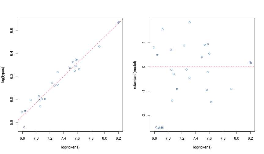
Heaps’ Law
The analysis tells us that Heap’s law accurately characterizes the lexical diversity (type-to-token ratio) for the main chapters in The Wizard of Oz. The number of unique types grows roughly as the number of tokens raised to the power 0.6.
The one chapter with an unusually low lexical diversity is Chapter 16. This chapter contains mostly dialogue between Oz and Dorothy’s simple-minded companions (the Scarecrow, Tin Woodman, and Lion).
Term statistics
Counts and prevalence
We get term statistics using the term_stats function:
term_stats(data) term count support
1 the 2922 24
2 and 1661 24
3 to 1108 24
4 of 824 24
5 you 489 24
6 in 478 24
7 dorothy 345 24
8 so 307 24
9 with 271 24
10 had 263 24
11 is 260 24
12 at 253 24
13 when 158 24
14 up 106 24
15 again 87 24
16 a 803 23
17 was 501 23
18 he 453 23
19 it 420 23
20 her 410 23
⋮ (2878 rows total)This returns a data frame with each row giving the count and support for each term. The “count” is the total number of occurrences of the term in the corpus. The “support” is the number of texts containing the term. In the output above, we can see that “the” is the most common term, appearing 2922 times total in all 24 chapters. The pronoun “her” is the 20th most common term, appearing in all but one chapter.
The most common words are English function words, commonly known as “stop” words. We can exclude these terms from the tally using the subset argument.
term_stats(data, subset = !term %in% stopwords_en) term count support
1 dorothy 345 24
2 said 332 23
3 little 139 22
4 one 125 22
5 asked 114 22
6 came 104 22
7 back 98 22
8 girl 93 22
9 toto 90 22
10 get 85 22
11 now 82 22
12 answered 78 22
13 scarecrow 217 21
14 upon 85 21
15 shall 82 21
16 go 72 21
17 looked 61 21
18 time 43 21
19 great 138 20
20 head 90 20
⋮ (2734 rows total)The character names “dorothy”, “toto”, and “scarecrow” show up at the top of the list of the most common terms.
Higher-order n-grams
Beyond searching for single-type terms, we can also search for multi-type terms (“n-grams”).
term_stats(data, ngrams = 5) term count support
1 scarecrow and the tin woodman 13 9
2 the scarecrow and the tin 13 9
3 the wicked witch of the 20 7
4 the road of yellow brick 12 7
5 wicked witch of the west 12 6
6 soldier with the green whiskers 8 6
7 the soldier with the green 8 6
8 the tin woodman and the 7 6
9 send me back to kansas 6 6
10 to get back to kansas 7 5
11 heart said the tin woodman 5 5
12 the guardian of the gates 10 4
13 in the middle of the 8 4
14 wicked witch of the east 8 4
15 until they came to the 6 4
16 to the land of the 5 4
17 and the tin woodman and 4 4
18 and the tin woodman were 4 4
19 in the midst of a 4 4
20 tin woodman and the lion 4 4
⋮ (38339 rows total)The types argument allows us to request the component types in the result:
term_stats(data, ngrams = 3, types = TRUE) term type1 type2 type3 count support
1 the tin woodman the tin woodman 112 18
2 said the scarecrow said the scarecrow 36 16
3 the emerald city the emerald city 53 14
4 the scarecrow and the scarecrow and 30 14
5 back to kansas back to kansas 28 14
6 as soon as as soon as 17 13
7 and the lion and the lion 24 12
8 the little girl the little girl 21 12
9 and the tin and the tin 19 12
10 and the scarecrow and the scarecrow 21 11
11 the lion and the lion and 19 11
12 the wicked witch the wicked witch 56 10
13 said the tin said the tin 19 10
14 the cowardly lion the cowardly lion 19 10
15 the land of the land of 19 10
16 they came to they came to 19 10
17 tin woodman and tin woodman and 18 10
18 scarecrow and the scarecrow and the 17 10
19 get back to get back to 15 10
20 asked the scarecrow asked the scarecrow 10 10
⋮ (32730 rows total)Here are the most common 2-, 3-grams starting with “dorothy”, where the second type is not a function word
term_stats(data, ngrams = 2:3, types = TRUE,
           subset = type1 == "dorothy" & !type2 %in% stopwords_en)
term type1 type2 type3 count support
1 dorothy said dorothy said <NA> 7 6
2 dorothy went dorothy went <NA> 6 6
3 dorothy looked dorothy looked <NA> 6 5
4 dorothy saw dorothy saw <NA> 5 5
5 dorothy walked dorothy walked <NA> 4 4
6 dorothy went to dorothy went to 4 4
7 dorothy asked dorothy asked <NA> 3 3
8 dorothy found dorothy found <NA> 3 3
9 dorothy looked at dorothy looked at 3 3
10 dorothy picked dorothy picked <NA> 3 3
11 dorothy sat dorothy sat <NA> 3 3
12 dorothy thought dorothy thought <NA> 3 3
13 dorothy put dorothy put <NA> 3 2
14 dorothy stood dorothy stood <NA> 3 2
15 dorothy answered dorothy answered <NA> 2 2
16 dorothy ate dorothy ate <NA> 2 2
17 dorothy awoke dorothy awoke <NA> 2 2
18 dorothy awoke the dorothy awoke the 2 2
19 dorothy can dorothy can <NA> 2 2
20 dorothy carried dorothy carried <NA> 2 2
⋮ (270 rows total)Searching for terms
Now that we have identified common terms, we might be interested in seeing where they appear. For this, we use the text_locate function.
Here are all instances of the term “dorothy looked”:
text_locate(data, "dorothy looked") text before instance after
1 ch02 …t from\nunder a block of wood."\n\n Dorothy looked , and gave a little cry of fright. …
2 ch05 …as if he could not stir at all.\n\n Dorothy looked at him in amazement, and so did th…
3 ch12 … a loud cry of fear, and then, as\n Dorothy looked at her in wonder, the Witch began …
4 ch14 …ll the mice hurrying after her.\n\n Dorothy looked inside the Golden Cap and saw some…
5 ch14 …the Monkey King finished his story Dorothy looked down and saw the\ngreen, shining w…
6 ch16 …ly he went back to his friends.\n\n Dorothy looked at him curiously. His head was qu…Note that we match against the type of the token, not the raw token itself, so we are able to detect capitalized “Dorothy”. This is especially useful when we want to search for a stemmed token. Here are all instances of tokens that stem to “scream”:
text_locate(data, "scream", stemmer = "en") # english stemmer text before instance after
1 ch01 …y the child's laughter that she would scream \nand press her hand upon her heart wh…
2 ch01 …ose at hand.\n\n"Quick, Dorothy!" she screamed . "Run for the cellar!"\n\nToto jumpe…
3 ch07 …oud\nand terrible a roar that Dorothy screamed and the Scarecrow fell over\nbackward…
4 ch12 …way.\n\n"See what you have done!" she screamed . "In a minute I shall melt\naway."\n…
5 ch17 … air without her.\n\n"Come back!" she screamed . "I want to go, too!"\n\n"I can't co…If we would like, we can search for multiple phrases at the same time:
text_locate(data, c("wicked witch", "toto", "oz")) text before instance after
1 ch01 …olemn, and rarely spoke.\n\nIt was Toto that made Dorothy laugh, and saved …
2 ch01 … gray\nas her other surroundings. Toto was not gray; he was a little black…
3 ch01 …ther side of his funny, wee nose. Toto played all day long, and\nDorothy p…
4 ch01 …l. Dorothy stood in the door with Toto in her arms, and looked at\nthe sky…
5 ch01 …creamed. "Run for the cellar!"\n\n Toto jumped out of Dorothy's arms and hi…
6 ch01 …small, dark\nhole. Dorothy caught Toto at last and started to follow her a…
7 ch01 …ently, like a baby in a cradle.\n\n Toto did not like it. He ran about the …
8 ch01 …to\nsee what would happen.\n\nOnce Toto got too near the open trap door, an…
9 ch01 …l. She crept to the hole,\ncaught Toto by the ear, and dragged him into th…
10 ch01 …er bed, and lay down upon it; and\n Toto followed and lay down beside her.\n…
11 ch02 …and wonder what had happened; and\n Toto put his cold little nose into her f…
12 ch02 … She sprang from her bed and with Toto at her heels ran\nand opened the do…
13 ch02 …teful to you for having killed the Wicked Witch of the\nEast, and for setting our p…
14 ch02 …ss, and saying she had\nkilled the Wicked Witch of the East? Dorothy was an innoce…
15 ch02 …e?" asked Dorothy.\n\n"She was the Wicked Witch of the East, as I said," answered t…
16 ch02 … this land of the East\n where the Wicked Witch ruled."\n\n"Are you a Munchkin?" as…
17 ch02 …e me. I am not as powerful as the Wicked Witch was who\nruled here, or I should ha…
18 ch02 …ly four witches in all the Land of Oz , and two of them,\nthose who live i…
19 ch02 …lled one of them, there is but one Wicked Witch \nin all the Land of Oz--the one who…
20 ch02 …e Wicked Witch\nin all the Land of Oz --the one who lives in the West."\n…
⋮ (303 rows total)We can also request that the results be returned in random order, using the text_sample() function. This function takes the results from text_locate() and randomly orders the rows; this is useful for inspecting a random sample of the matches:
text_sample(data, c("wicked witch", "toto", "oz")) text before instance after
1 ch17 … just touched the\nground.\n\nThen Oz got into the basket and said to all…
2 ch06 …e so tender of?"\n\n"He is my dog, Toto ," answered Dorothy.\n\n"Is he made …
3 ch10 …hy do you wish to see the terrible Oz ?" asked the man.\n\n"I want him to …
4 ch12 …iends.\n\n"Which road leads to the Wicked Witch of the West?" asked Dorothy.\n\n"Th…
5 ch24 …aid Dorothy gravely. "And here is Toto , too.\nAnd oh, Aunt Em! I'm so gla…
6 ch05 …as scarcely enough for herself and Toto for the day.\n\nWhen she had finish…
7 ch17 …then a strip of emerald green; for Oz had a fancy to make the balloon\nin…
8 ch18 …hould like to cry a little because Oz is gone,\nif you will kindly wipe a…
9 ch12 …would cry bitterly for hours, with Toto sitting at her feet and\nlooking in…
10 ch12 …e out of the dark sky to show\nthe Wicked Witch surrounded by a crowd of monkeys, e…
11 ch02 …lled one of them, there is but one Wicked Witch \nin all the Land of Oz--the one who…
12 ch23 …he Emerald City," he replied, "for Oz has made me\nits ruler and the peop…
13 ch03 …"If you will come with me I'll ask Oz to do all he can for\nyou."\n\n"Tha…
14 ch13 … was much pleased to hear that the Wicked Witch had\nbeen melted by a bucket of wat…
15 ch10 …hat pleases him. But who the real Oz \nis, when he is in his own form, no…
16 ch15 …into the Throne Room\nof the Great Oz .\n\nOf course each one of them expe…
17 ch11 …e Wicked Witch of the East," said\n Oz .\n\n"That just happened," returned …
18 ch14 …ey sat down and looked at her, and Toto found that\nfor the first time in h…
19 ch18 … crossed the\ndesert, unless it is Oz himself."\n\n"Is there no one who c…
20 ch10 …," said Dorothy, "to see the Great Oz ."\n\n"Oh, indeed!" exclaimed the ma…
⋮ (303 rows total)Other functions allow counting term occurrences, testing for whether a term appears in a text, and getting the subset of texts containing a term:
text_count(data, "the great oz")ch01 ch02 ch03 ch04 ch05 ch06 ch07 ch08 ch09 ch10 ch11 ch12 ch13 ch14 ch15 ch16 ch17 ch18 ch19
0 0 3 1 1 1 0 0 0 5 3 1 0 0 2 0 0 0 0
ch20 ch21 ch22 ch23 ch24
0 0 0 0 0 text_detect(data, "the great oz") ch01 ch02 ch03 ch04 ch05 ch06 ch07 ch08 ch09 ch10 ch11 ch12 ch13 ch14 ch15
FALSE FALSE TRUE TRUE TRUE TRUE FALSE FALSE FALSE TRUE TRUE TRUE FALSE FALSE TRUE
ch16 ch17 ch18 ch19 ch20 ch21 ch22 ch23 ch24
FALSE FALSE FALSE FALSE FALSE FALSE FALSE FALSE FALSE text_subset(data, "the great oz")ch03
"When Dorothy was left alone she began to feel hungry. So she went to\nthe cupboard and cut …"
ch04
"After a few hours the road began to be rough, and the walking grew so\ndifficult that the Sc…"
ch05
"When Dorothy awoke the sun was shining through the trees and Toto had\nlong been out chasing…"
ch06
"All this time Dorothy and her companions had been walking through the\nthick woods. The roa…"
ch10
"It was some time before the Cowardly Lion awakened, for he had lain\namong the poppies a lon…"
ch11
"Even with eyes protected by the green spectacles, Dorothy and her\nfriends were at first daz…"
ch12
"The soldier with the green whiskers led them through the streets of the\nEmerald City until …"
ch15
"The four travelers walked up to the great gate of Emerald City and rang\nthe bell. After ri…"Segmenting text
Sentences and blocks of tokens
Corpus can split text into blocks of sentences or tokens using the text_split function. By default, this function splits into sentences. Here, for example, are the last 10 sentences in the book:
tail(text_split(data), 10) parent index text
2207 ch23 62 Dorothy stood up and found she was in her stocking-feet.
2208 ch23 63 For the\nSilver Shoes had fallen off in her flight through the air, and were…
2209 ch24 1 Aunt Em had just come out of the house to water the cabbages when she\nlooke…
2210 ch24 2 "My darling child!"
2211 ch24 3 she cried, folding the little girl in her arms and\ncovering her face with k…
2212 ch24 4 "Where in the world did you come from?"\n\n
2213 ch24 5 "From the Land of Oz," said Dorothy gravely.
2214 ch24 6 "And here is Toto, too.\n
2215 ch24 7 And oh, Aunt Em!
2216 ch24 8 I'm so glad to be at home again!" The result of text_split is a data frame, with one row for each segment identifying the parent text (as a factor), the index of the segment in the parent text (an integer), and the segment text.
The second argument to text_split specifies, the units, “sentences” or “tokens”. The third argument specifies the maximum segment size, defaulting to one. Each text gets divided into approximately equal-sized segments, with no segment being larger than the specified size.
Here is an example of splitting two texts into segments of size at most four tokens.
text_split(c("the wonderful wizard of oz", paste(LETTERS, collapse = " ")),
           "tokens", 4)
parent index text
1 1 1 the wonderful wizard
2 1 2 of oz
3 2 1 A B C D
4 2 2 E F G H
5 2 3 I J K L
6 2 4 M N O P
7 2 5 Q R S T
8 2 6 U V W
9 2 7 X Y Z Application: Witch tracking
We can combine text_split with text_count to measure the occurrences rates for the term “witch” over the course of the novel. Here, the chunks have varying sizes, so we look at the rates rather than the raw counts.
chunks <- text_split(data, "tokens", 500)
size <- text_ntoken(chunks)

unit <- 1000 # rate per 1000 tokens
count <- text_count(chunks, "witch")
rate <-  count / size * unit

i <- seq_along(rate)
plot(i, rate, type = "l", xlab = "Segment",
     ylab = "Rate \u00d7 1000",
     main = paste(dQuote("witch"), "Occurrences"), col = 2)
points(i, rate, pch = 16, cex = 0.5, col = 2)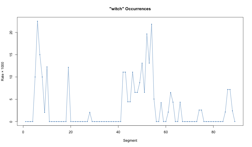
‘witch’ Occurences
We can see Dorothy’s house landing on the Wicked Witch of the East in the and the subsequent fallout in the beginning of the novel. Around segment 40, we see the events surrounding Dorothy’s battle with the Wicked Witch of the West. At the end of the novel, we see the Good Witch of the South appearing to help Dorothy get home.
Term frequency matrix
Many downstream text analysis tasks require tabulating a matrix of text-term occurrence counts. We can get such a matrix using the term_matrix function:
x <- term_matrix(data)
dim(x)
[1] 24 2878This function returns a sparse matrix object from the Matrix package. In the default usage, the rows of the matrix correspond to texts, and the columns correspond to terms. For a “term-by-document” matrix, you can use the transpose option:
xt <- term_matrix(data, transpose = TRUE)You can include n-grams in the result if you would like:
x3 <- term_matrix(data, ngrams = 1:3) # 1-, 2-, and 3-gramsOr, you can specify the columns to include in the matrix
(x <- term_matrix(data, select = c("dorothy", "toto", "wicked witch", "the great oz")))24 x 4 sparse Matrix of class "dgCMatrix"
dorothy toto wicked witch the great oz
ch01 15 10 . .
ch02 31 3 8 .
ch03 24 14 3 3
ch04 8 3 . 1
ch05 13 4 5 1
ch06 12 9 . 1
ch07 13 4 . .
ch08 16 5 1 .
ch09 5 5 . .
ch10 18 6 . 5
ch11 32 1 11 3
ch12 33 7 19 1
ch13 11 1 2 .
ch14 15 2 2 .
ch15 18 2 6 2
ch16 3 . . .
ch17 10 2 . .
ch18 15 . . .
ch19 8 2 . .
ch20 20 3 . .
ch21 4 2 . .
ch22 7 2 . .
ch23 12 2 1 .
ch24 2 1 . .The columns of x will be in the same order as specified by the select argument. Note that we can request higher-order n-grams.
Emotion lexicon
Corpus provides a lexicon of terms connoting emotional affect, the WordNet Affect Lexicon.
affect_wordnet term pos category emotion
1 jollity NOUN Joy Positive
2 joviality NOUN Joy Positive
3 chaff VERB Joy Positive
4 kid VERB Joy Positive
5 banter VERB Joy Positive
6 jolly VERB Joy Positive
7 merry ADJ Joy Positive
8 jovial ADJ Joy Positive
9 jolly ADJ Joy Positive
10 jocund ADJ Joy Positive
11 gay ADJ Joy Positive
12 mirthful ADJ Joy Positive
13 riotously ADV Joy Positive
14 exuberantly ADV Joy Positive
15 expansively ADV Joy Positive
16 ebulliently ADV Joy Positive
17 exuberance NOUN Joy Positive
18 lightheartedness NOUN Joy Positive
19 carefreeness NOUN Joy Positive
20 lightsomeness NOUN Joy Positive
⋮ (1641 rows total)This lexicon classifies a large set of terms correlated with emotional affect into four main categories: “Positive”, “Negative”, “Ambiguous”, and “Neutral”, and a variety of sub-categories. Here is a summary:
summary(affect_wordnet) term pos category emotion
Length:1641 NOUN:532 Dislike:338 Positive :541
Class :character ADJ :642 Sadness:199 Negative :978
Mode :character VERB:267 Joy :191 Neutral : 32
ADV :200 Fear :171 Ambiguous: 90
Liking :106
Anxiety: 97
(Other):539 Here are the term counts broken down by category:
with(affect_wordnet, table(category, emotion)) emotion
category Positive Negative Neutral Ambiguous
Joy 191 0 0 0
Love 40 0 0 0
Affection 20 0 0 0
Liking 106 0 0 0
Enthusiasm 27 0 0 0
Gratitude 8 0 0 0
Pride 22 0 0 0
Levity 14 0 0 0
Calmness 64 0 0 0
Fearlessness 19 0 0 0
Expectation 7 0 0 18
Fear 7 151 0 13
Hope 16 0 0 0
Sadness 0 199 0 0
Dislike 0 338 0 0
Ingratitude 0 2 0 0
Shame 0 82 0 0
Compassion 0 29 0 0
Humility 0 19 0 0
Despair 0 47 0 0
Anxiety 0 97 0 0
Daze 0 14 0 0
Apathy 0 0 20 0
Unconcern 0 0 12 0
Gravity 0 0 0 11
Surprise 0 0 0 8
Agitation 0 0 0 27
Pensiveness 0 0 0 13Terms can appear in multiple categories, or with multiple parts of speech.
# some duplicate terms
subset(affect_wordnet, term %in% c("caring", "chill", "hopeful"))
term pos category emotion
209 caring NOUN Love Positive
248 caring ADJ Affection Positive
309 caring ADJ Liking Positive
462 chill VERB Calmness Positive
520 chill NOUN Fear Positive
526 hopeful ADJ Hope Positive
626 chill NOUN Fear Negative
628 chill VERB Fear Negative
1337 caring ADJ Compassion Negative
1624 hopeful ADJ Expectation AmbiguousThe term “chill”, for example, is listed as denoting both positive calmness and negative fear, among other emotional affects.
Application: Emotion in The Wizard of Oz
Overview
For our final application, we will track emotion word usage over the course of The Wizard of Oz. We will do this by segmenting the novel into small chunks, and then measure the occurrence rates of emotion words in these chunks.
Lexicon
We will first need a lexicon of emotion words. We will take as a starting point the WordNet-Affect lexicon, but we will remove “Neutral” emotion words.
affect <- subset(affect_wordnet, emotion != "Neutral")
affect$emotion <- droplevels(affect$emotion) # drop the unused "Neutral" level
affect$category <- droplevels(affect$category) # drop unused categories
Rather than blindly applying the lexicon, we first check to see what the most common emotion terms are.
term_stats(data, subset = term %in% affect$term) term count support
1 down 93 22
2 great 138 20
3 good 74 20
4 like 64 19
5 heart 67 16
6 yellow 33 14
7 near 20 14
8 glad 19 14
9 afraid 29 13
10 still 20 12
11 surprise 15 12
12 happy 15 11
13 wicked 72 10
14 low 15 10
15 close 13 10
16 terrible 27 9
17 sorry 14 9
18 frightened 13 9
19 blue 21 8
20 dark 16 8
⋮ (168 rows total)A few terms jump out as unusual: “yellow” is probably for the yellow brick road; “down” and “near” probably do not evoke emotions. We can inspect the usages of the most common terms using the text_locate function, which shows these terms in context.
text_sample(data, "down") text before instance after
1 ch12 …to and\nthe Lion were tired, and lay down upon the grass and fell asleep, with…
2 ch11 …d the night moving his joints up and down \nto make sure they kept in good worki…
3 ch08 …rew heavy\nand she felt she must sit down to rest and to sleep.\n\nBut the Tin …
4 ch22 …uck by a cannon ball.\n\nDorothy ran down and helped the Scarecrow to his feet,…
5 ch04 …stuffed with straw.'\nThen he hopped down at my feet and ate all the corn he wa…
6 ch19 …\nunder the first branches they bent down and twined around him, and the\nnext …
7 ch02 …aw.\n\nThe cyclone had set the house down very gently--for a cyclone--in the\nm…
8 ch22 …s safely\nover the hill and set them down in the beautiful country of the\nQuad…
9 ch03 …in a friendly way. Then she climbed down from the fence\nand walked up to it, …
10 ch04 …ried leaves in one\ncorner. She lay down at once, and with Toto beside her soo…
11 ch17 …m he greeted her pleasantly:\n\n"Sit down , my dear; I think I have found the wa…
12 ch14 …ould\ndo. At his word the band flew down and seized Quelala, carried him in\nt…
13 ch07 …Dorothy with dry leaves when she lay down to sleep.\nThese kept her very snug a…
14 ch10 …surprised at this answer that he sat down to think it\nover.\n\n"It has been ma…
15 ch02 …hall have them to wear." She reached down and picked up\nthe shoes, and after s…
16 ch07 …d not leap across it.\n\nSo they sat down to consider what they should do, and …
17 ch20 … he found in the\nforest Dorothy lay down and slept, for she was tired by the l…
18 ch12 … thanked him for saving them and sat down \nto breakfast, after which they start…
19 ch12 …k to their work, after which she sat down to\nthink what she should do next. S…
20 ch07 …t is certain. Neither can\nwe climb down into this great ditch. Therefore, if…
⋮ (93 rows total)Here, we use the text_sample() instead of text_locate() to return the matches in random order. Since we are only looking at a subset of the matches, we use this option to ensure that we don’t make conclusions about these words using a biased sample. Using text_locate(), we would would only see the matches at the beginning of the novel.
It looks like “down” is mostly used as a preposition, not an emotion. We will exclude it form the lexicon.
text_sample(data, "good") text before instance after
1 ch11 …ued the voice.\n\n"That is where the Good Witch of the North kissed me when she…
2 ch15 … Witches of the North and South were good , and I knew\nthey would do me no harm…
3 ch10 …f\neverything, and was glad to get a good supper again.\n\nThe woman now gave D…
4 ch11 … and down\nto make sure they kept in good working order. The Lion would have\n…
5 ch04 …brains in your head you would be as good a man as any of them, and a\nbetter m…
6 ch15 …"Just to amuse myself, and keep the good people busy, I ordered them to\nbuild…
7 ch05 …ey were quite free from rust\nand as good as new.\n\nThe Tin Woodman gave a sig…
8 ch22 …leader to Dorothy;\n"so good-bye and good luck to you."\n\n"Good-bye, and thank…
9 ch19 …knew how to give me brains, and very good brains, too," said the\nScarecrow.\n…
10 ch21 … O King of Beasts! You have come in good time to fight our\nenemy and bring pe…
11 ch15 …ewels and precious metals, and every good thing\nthat is needed to make one hap…
12 ch10 … And we have been told that Oz is a good \nWizard."\n\n"So he is," said the gre…
13 ch23 … her\nloving comrades.\n\nGlinda the Good stepped down from her ruby throne to …
14 ch02 …wered the little woman. "But I am a good witch, and\nthe people love me. I am…
15 ch18 … until she starts back to Kansas for good and all."\n\n"Thank you," said Doroth…
16 ch19 … lovely City, and everyone has\nbeen good to me. I cannot tell you how gratefu…
17 ch07 …amed of the Emerald City, and of the good \nWizard Oz, who would soon send her b…
18 ch14 …owed by all his band.\n\n"That was a good ride," said the little girl.\n\n"Yes,…
19 ch15 …Dorothy," said the Lion gravely.\n\n" Good gracious!" exclaimed the man, and he …
20 ch14 …s never known to hurt anyone who was good . Her name\nwas Gayelette, and she li…
⋮ (74 rows total)“Good” seems to be an appropriate emotion work, evoking positive affection or love. We will keep it in the lexicon.
text_sample(data, "heart") text before instance after
1 ch15 …w.\n\n"And you promised to give me a heart ," said the Tin Woodman.\n\n"And you p…
2 ch09 …," replied the Woodman. "I have no\n heart , you know, so I am careful to help al…
3 ch18 …n for the man who gave\nme my lovely heart . I should like to cry a little becau…
4 ch14 …ywhere at all."\n\nThen Dorothy lost heart . She sat down on the grass and looke…
5 ch07 …ures\nfrightened me so badly that my heart is beating yet."\n\n"Ah," said the Ti…
6 ch05 …; but no one\ncan love who has not a heart , and so I am resolved to ask Oz to gi…
7 ch06 …y.\nBut whenever there is danger, my heart begins to beat fast."\n\n"Perhaps you…
8 ch15 …t a murmur, if you will\ngive me the heart ."\n\n"Very well," answered Oz meekly.…
9 ch19 …aid the Tin Woodman, as he\nfelt his heart rattling around in his breast.\n\n"He…
10 ch08 …ke them better."\n\n"If I only had a heart , I should love them," added the Tin W…
11 ch11 …d, gruffly: "If you indeed desire a\n heart , you must earn it."\n\n"How?" asked t…
12 ch11 …I am such a fool."\n\n"I haven't the heart to harm even a Witch," remarked the T…
13 ch05 … why he was so anxious to get a\nnew heart .\n\n"All the same," said the Scarecro…
14 ch18 …oodman, "am well-pleased with my new heart ;\nand, really, that was the only thin…
15 ch15 …w it, you are in\nluck not to have a heart ."\n\n"That must be a matter of opinio…
16 ch23 …ng\nlittle girl.\n\n"Bless your dear heart ," she said, "I am sure I can tell you…
17 ch16 …"Oh, very!" answered Oz. He put the heart in the Woodman's breast and\nthen rep…
18 ch05 …I shall ask for brains instead of\na heart ; for a fool would not know what to do…
19 ch01 … scream\nand press her hand upon her heart whenever Dorothy's merry voice\nreach…
20 ch16 …e\nin your breast, so I can put your heart in the right place. I hope it\nwon't…
⋮ (67 rows total)“Heart” is mostly used as an object (noun), not an emotion meaning compassion. The Tin Woodman’s search for a heart is a central plot of the novel, so it is not surprising that the term shows up frequently. We can look for co-occurrences of “heart” with “woodman”:
loc <- text_locate(data, "heart")
before <- text_detect(text_sub(loc$before, -25, -1), "woodman")
after <- text_detect(text_sub(loc$after, 1, 25), "woodman")
summary(before | after)
Mode FALSE TRUE
logical 16 51 “Woodman” appears within 25 tokens of “heart” in in 45 of the 67 contexts where the latter word appears.
The decision of whether to include or exclude “heart” is a difficult judgment call. Most of the time it appears, it describes an object, not an emotion. Still, that object does have an emotional association. I’m deciding to include “heart”, but this is not a clear-cut decision.
We can also inspect the first token after each appearance of “yellow”:
term_stats(text_sub(text_locate(data, "yellow")$after, 1, 1)) term count support
1 brick 16 16
2 and 3 3
3 winkies 3 3
4 bricks 2 2
5 castle 2 2
6 daisies 1 1
7 flowers 1 1
8 in 1 1
9 land 1 1
10 road-bed 1 1
11 rooms 1 1
12 wildcat 1 1Over half the time, “yellow” prefaces “brick” or “bricks”, and otherwise it describes objects. It does not describe or evoke emotion, and we should exclude it from the lexicon.
Similar analysis not shown here indicates that “great” is mostly used to describe size, not positive enthusiasm; “like” is often used to mean “similar to”, not “affection for”; “blue” is mostly used as a color, not an emotion.
All of this analysis shows that we should probably exclude some of the common terms from the lexicon.
affect <- subset(affect, !term %in% c("down", "great", "like", "yellow", "near", "low", "blue"))Term emotion matrix
Now that we have a lexicon, our plan is to segment the text into smaller chunks and then compute the emotion occurrence rates in each chunk, broken down by category (“Positive”, “Negative”, or “Ambiguous”).
To facilitate the rate computations, we will form a term-by-emotion rate for the lexicon:
term_scores <- with(affect, unclass(table(term, emotion)))
head(term_scores)
emotion
term Positive Negative Ambiguous
abase 0 2 0
abash 0 1 0
abashed 0 1 0
abashment 0 1 0
abhor 0 1 0
abhorrence 0 1 0Here, term_scores is a matrix with entry (i,j) indicating the number of times that term i appeared in the affect lexicon with emotion j.
We re-classify any term appearing in two or more categories as ambiguous:
ncat <- rowSums(term_scores > 0)
term_scores[ncat > 1, c("Positive", "Negative", "Ambiguous")] <- c(0, 0, 1)
At this point, every term is in one category, but the score for the term could be 2, 3, or more, depending on the number of sub-categories the term appeared in. We replace these larger values with one.
term_scores[term_scores > 1] <- 1Segmenting chapters into smaller chunks
To compute emotion occurrence rates, we start by splitting each chapter into equal-sized segments of at most 500 tokens. The specific size of 500 tokens is somewhat arbitrary, but not entirely so. We want the segments to be large enough so that our rate estimates are reliable, but not so large that the emotion usage is heterogeneous within the segment.
chunks <- text_split(data, "tokens", 500)Within a chapter, the segments all have approximately the same size. However, since the chapters have different lengths, there is some variation in segment size across chapters:
(n <- text_ntoken(chunks)) [1] 381 381 380 401 400 400 400 400 489 489 489 488 478 478 478 411 411 411 411 410 500 499
[23] 499 450 450 449 449 482 482 481 481 461 461 461 488 488 487 487 451 451 451 451 451 451
[45] 451 451 459 459 459 458 458 458 458 458 396 396 396 472 471 471 471 460 460 460 460 460
[67] 460 461 460 384 384 383 388 387 387 337 337 337 500 500 500 446 445 466 465 417 417 416
[89] 74(If we wanted equal sized segments, we could have concatenated the chapters together and then split the combined text. The disadvantage of this approach is that some segments would be split across multiple chapters.)
Computing emotion rates
For the count of each emotion category in each segment, we form a text-by-term matrix of counts, and then multiply this by the term-by-emotion score matrix.
x <- term_matrix(chunks, select = rownames(term_scores))
text_scores <- x %*% term_scores
For the occurrence rates, we divide the counts by the segment sizes. We then multiply by 1000 so that rates are given as occurrences per 1000 tokens.
# compute the rates per 1000 tokens
unit <- 1000
rate <- list(pos = text_scores[, "Positive"] / n * unit,
             neg = text_scores[, "Negative"] / n * unit,
             ambig = text_scores[, "Ambiguous"] / n * unit)
rate$total <- rate$pos + rate$neg + rate$ambig
We use the binomial variance formula to get the standard errors:
# compute the standard errors
se <- lapply(rate, function(r) sqrt(r * (unit - r) / n))
This is a crude estimate that makes some independence assumptions, but it gives a reasonable approximation of the uncertainty associated with our measured rates.
Plotting the results
We plot the four rate curves as time series. Our main focus is on the total emotion usage. For this curve, we also put a horizontal dashed line at its mean, and we indicating the “interesting” segments, those that appear more than two standard deviations away from the main, by putting error bars on these points.
# set up segment IDs
i <- seq_len(nrow(chunks))

# set the plot margins, with extra space below the plot
par(mar = c(4, 4, 11, 9) + 0.1, las = 1)

# set up the plot coordinates; put labels but no axes
xlim <- range(i - 0.5, i + 0.5)
ylim <- range(0, rate$total + se$total, rate$total - se$total)
plot(xlim, ylim, type = "n", xlab = "Segment", ylab = "Rate \u00d7 1000", axes = FALSE,
     xaxs = "i")
usr <- par("usr") # get the user coordinates for later

# put tick marks at multiples of 5 on the x axis; labels at multiples of 10
axis(1, at = i[i %% 5 == 0], labels = FALSE)
axis(1, at = i[i %% 10 == 0], labels = TRUE)

# defaults for the y axis
axis(2)

# put vertical lines at chapter boundaries
abline(v = tapply(i, chunks$parent, min) - 0.5, col = "gray")

# put chapter titles above the plot
labels <- data$title
at <- tapply(i, chunks$parent, mean)

# (adapted from https://www.r-bloggers.com/rotated-axis-labels-in-r-plots/)
text(at, usr[4] + 0.01 * diff(usr[3:4]),
     labels = labels, adj = 0, srt = 45, cex = 0.8, xpd = TRUE)

# frame the plot
box()

# colors for the different emotions, from RColorBrewer::brewer.pal(3, "Set2")
col <- c(total = "#000000", pos = "#FC8D62", neg = "#8DA0CB", ambig = "#66C2A5")

# add a legend on the right hand side
legend(usr[2] + 0.015 * diff(usr[1:2]), usr[3] + 0.8 * diff(usr[3:4]),
       legend = c("Total", "Positive", "Negative", "Ambiguous"),
       title = expression(bold("Emotion")),
       fill = col[c("total", "pos", "neg", "ambig")],
       cex = 0.8, xpd = TRUE)

# for the total rate, put a dashed line at the mean rate
abline(h = mean(rate$total), lty = 2, col = col[["total"]])

# plot each rate type
for (t in c("ambig", "neg", "pos", "total")) {
    r <- rate[[t]]
    s <- se[[t]]
    cl <- col[[t]]

    # add lines and points
    lines(i, r, col = cl)
    points(i, r, col = cl, pch = 16, cex = 0.5)

    # for the total, put standard errors around interesting points
    if (t == "total") {
        # "interesting" defined as rate >2 sd away from mean
        int <- abs((r - mean(r)) / sd(r)) > 2

        segments(i[int], (r - s)[int], i[int], (r + s)[int], col = cl)
        segments((i - .2)[int], (r - s)[int], (i + .2)[int], (r - s)[int], col = cl)
        segments((i - .2)[int], (r + s)[int], (i + .2)[int], (r + s)[int], col = cl)
    }
}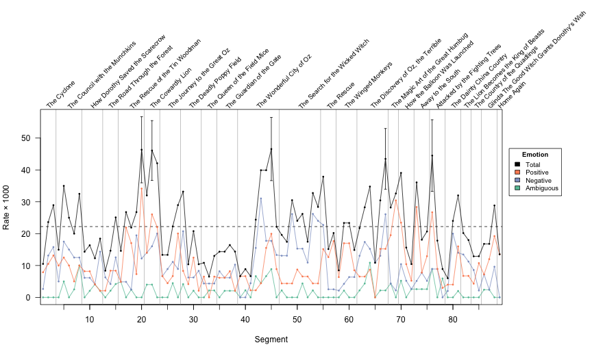
Emotion in Oz
Discussion
This is a crude measurement, but it appears to give a reasonable approximation of the emotional dynamics of the novel. There are some interesting dynamics to the “Positive” and “Negative” emotions, but I’m going to focus on the “Total” emotion.
There are five segments where the rate of emotion word usage is two or more standard deviations above the mean for the rest of the novel. In all five cases, these are statistically significant differences (more than two standard errors above the mean). The first two interesting segments are when Dorothy meets the Tin Woodman and the Cowardly Lion. The next is when the Dorothy and her companions meet the Great Oz for the first time and he tasks them with defeating the Wicked Witch of the West; this is the point in the novel with the highest emotion word usage. The fourth interesting point is when Oz is revealed to be a common man, not a great wizard. The last emotional segment is when Dorothy and her companions leave the Emerald city feeling triumphant and hopeful.
Summary
The corpus library provides facilities for transforming texts into sequences of tokens and for computing the statistics of these sequences. The text_filter() function allows us to control the transformation from text to tokens. The text_stats() and term_stats() functions compute text- and term-level occurrence statistics. The text_locate() function and allow us to search for terms within texts. The term_matrix() function computes a text-by-term frequency matrix. These functions and their variants provide the building blocks for analyzing text.
For more information, check the other vignettes or the package documentation with library(help = "corpus").